Signal Processing - 101¶

In [1]:

!git clone https://github.com/amirberenji1995/damavand

!git clone https://github.com/amirberenji1995/damavand

fatal: destination path 'damavand' already exists and is not an empty directory.

In [2]:

!pip install -r damavand/requirements.txt

!pip install -r damavand/requirements.txt

Requirement already satisfied: certifi==2024.7.4 in /usr/local/lib/python3.11/dist-packages (from -r damavand/requirements.txt (line 1)) (2024.7.4)
Requirement already satisfied: charset-normalizer==3.3.2 in /usr/local/lib/python3.11/dist-packages (from -r damavand/requirements.txt (line 2)) (3.3.2)
Requirement already satisfied: idna==3.7 in /usr/local/lib/python3.11/dist-packages (from -r damavand/requirements.txt (line 3)) (3.7)
Requirement already satisfied: numpy==1.26.4 in /usr/local/lib/python3.11/dist-packages (from -r damavand/requirements.txt (line 4)) (1.26.4)
Requirement already satisfied: pandas==2.1.4 in /usr/local/lib/python3.11/dist-packages (from -r damavand/requirements.txt (line 5)) (2.1.4)
Requirement already satisfied: python-dateutil==2.9.0.post0 in /usr/local/lib/python3.11/dist-packages (from -r damavand/requirements.txt (line 6)) (2.9.0.post0)
Requirement already satisfied: pytz==2024.1 in /usr/local/lib/python3.11/dist-packages (from -r damavand/requirements.txt (line 7)) (2024.1)
Requirement already satisfied: rarfile==4.2 in /usr/local/lib/python3.11/dist-packages (from -r damavand/requirements.txt (line 8)) (4.2)
Requirement already satisfied: requests==2.32.3 in /usr/local/lib/python3.11/dist-packages (from -r damavand/requirements.txt (line 9)) (2.32.3)
Requirement already satisfied: scipy==1.13.1 in /usr/local/lib/python3.11/dist-packages (from -r damavand/requirements.txt (line 10)) (1.13.1)
Requirement already satisfied: six==1.16.0 in /usr/local/lib/python3.11/dist-packages (from -r damavand/requirements.txt (line 11)) (1.16.0)
Requirement already satisfied: tzdata==2024.1 in /usr/local/lib/python3.11/dist-packages (from -r damavand/requirements.txt (line 12)) (2024.1)
Requirement already satisfied: urllib3==2.2.2 in /usr/local/lib/python3.11/dist-packages (from -r damavand/requirements.txt (line 13)) (2.2.2)

1. Signal Processing: Unlocking Insights from Vibration Data¶

Vibration data from rotating machinery is a goldmine of information, but it's hidden in noise and complexity. Signal processing is the key to unlocking this information. Think of it as translating the machine's "language" of vibrations into a clear, understandable message about its health.

We start with the signal itself—a representation of vibration over time, either as a continuous analog wave or a discrete digital sequence. Signal processing then uses various techniques to enhance and analyze this signal:

• Time-domain analysis: Looking directly at the signal's shape over time. Think of it like reading a story—we look for sudden changes, repeating patterns, or unusual spikes.
• Frequency-domain analysis (FFT): Transforming the signal to see its hidden frequencies. This is like musical analysis—we identify the dominant notes (frequencies) that reveal the machine's internal workings and potential problems.
• Filtering: Cleaning up the signal by removing unwanted noise. This is like editing a recording—we remove background noise to hear the main instrument clearly.

By combining these techniques, we can extract crucial features from the vibration data, such as characteristic frequencies associated with specific faults, enabling early detection and diagnosis of problems. This allows for proactive maintenance, preventing costly breakdowns and ensuring operational efficiency. This notebook explores these techniques and how they are applied using [Package Name] to analyze vibration data and improve rotating machinery reliability.

2. Essential Theory¶

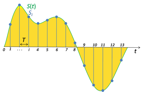
2.1 Sampling of Vibration Signals¶

Real-world vibration signals are continuous-time and analog. Digital processing requires sampling—converting the signal into a discrete-time sequence by measuring amplitude at regular intervals determined by the sampling frequency, f_s, with sampling interval T_s = 1/f_s.

2.2 Nyquist-Shannon Sampling Theorem¶

Aliasing is phenomena which causes higher frequencies to appear as lower ones in the sampled data.

To avoid information loss (aliasing), the sampling frequency must be at least twice the maximum frequency present in the signal (f_s ≥ 2f_max). Anti-aliasing filters are used before sampling to remove frequencies above f_max.

2.3 Leakage Error¶

Leakage error arises in frequency spectrum analysis when the analyzed signal's duration is not an integer multiple of its fundamental period. This discontinuity at the observation window's edges causes spectral energy to "leak" into adjacent frequency bins, blurring the true frequency components and distorting their amplitudes.

Windowing techniques (e.g., Hanning, Hamming) mitigate this by smoothly tapering the signal's ends, reducing the discontinuity and minimizing spectral leakage.

2.4 Modulation and Demodulation¶

Modulation modifies a carrier signal's properties using a message signal. In Amplitude Modulation (AM), the modulated signal is: s(t) = A_c[1 + m(t)]cos(2πf_ct), where A_c and f_c are the carrier's amplitude and frequency, and m(t) is the message signal.

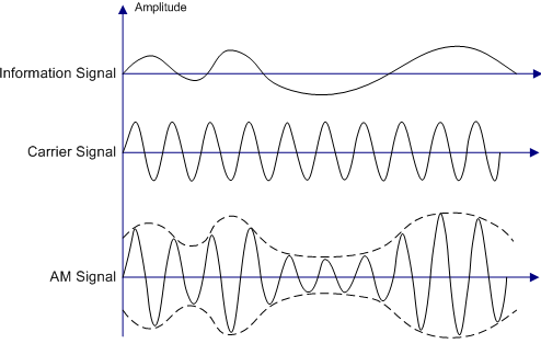
In RCM, machine speed variations modulate fault frequencies. Demodulation thecniques (etc. envelope extraction using Hilbert transform) recovers the message signal.

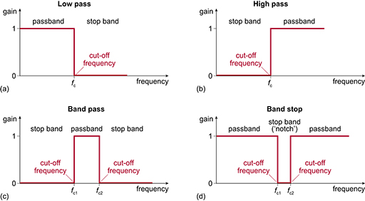
2.5 Frequency Filtering¶

Filtering selectively removes or attenuates specific frequency components. Common filter types include:

• Low-pass filters: Pass frequencies below a cutoff frequency and attenuate higher frequencies.
• High-pass filters: Pass frequencies above a cutoff frequency and attenuate lower frequencies.
• Band-pass filters: Pass frequencies within a specific band and attenuate frequencies outside this band.
• Band-stop filters (notch filters): Attenuate frequencies within a specific band and pass frequencies outside this band.

3. Signal Processing using Damavand¶

Damavand offers two main approaches to process vibration signals:

1. Applying transformations: Damavand facilitates the application of the most frequent signal processing transformations.
2. Fetaure extraction: In addition to the transformations, Damavand also supports the extraction of expert-defined features.

3.1 Transformations¶

3.1.0 Downloading and Mining the MFPT dataset¶

In [3]:

from damavand.damavand.datasets.downloaders import read_addresses, ZipDatasetDownloader
from damavand.damavand.datasets.digestors import MFPT
import pandas as pd

# Downloading the MFPT dataset
addresses = read_addresses()
downloader = ZipDatasetDownloader(addresses['MFPT'])
downloader.download_extract('MFPT.zip', 'MFPT/')

mfpt = MFPT('MFPT/MFPT Fault Data Sets/', [
    '1 - Three Baseline Conditions',
    '2 - Three Outer Race Fault Conditions',
    '3 - Seven More Outer Race Fault Conditions',
    '4 - Seven Inner Race Fault Conditions',
])

# Mining the dataset
mining_params = {
    97656: {'win_len': 16671, 'hop_len': 2000},
    48828: {'win_len': 8337, 'hop_len': 1000},
}
mfpt.mine(mining_params)

# Signal/Metadata split
df = pd.concat(mfpt.data[48828]).reset_index(drop = True)
signals, metadata = df.iloc[:, : - 4], df.iloc[:, - 4 :]

from damavand.damavand.datasets.downloaders import read_addresses, ZipDatasetDownloader from damavand.damavand.datasets.digestors import MFPT import pandas as pd # Downloading the MFPT dataset addresses = read_addresses() downloader = ZipDatasetDownloader(addresses['MFPT']) downloader.download_extract('MFPT.zip', 'MFPT/') mfpt = MFPT('MFPT/MFPT Fault Data Sets/', [ '1 - Three Baseline Conditions', '2 - Three Outer Race Fault Conditions', '3 - Seven More Outer Race Fault Conditions', '4 - Seven Inner Race Fault Conditions', ]) # Mining the dataset mining_params = { 97656: {'win_len': 16671, 'hop_len': 2000}, 48828: {'win_len': 8337, 'hop_len': 1000}, } mfpt.mine(mining_params) # Signal/Metadata split df = pd.concat(mfpt.data[48828]).reset_index(drop = True) signals, metadata = df.iloc[:, : - 4], df.iloc[:, - 4 :]

3.1.1 Envelope extraction (Hilbert transform)¶

Extracting the envelope of of signals.

In [4]:

from damavand.damavand.signal_processing.transformations import env

# Envelope extraction
signals_env = env(signals)

from damavand.damavand.signal_processing.transformations import env # Envelope extraction signals_env = env(signals)

3.1.2 Frequency spectrum extraction (Fast-Fourier Transform)¶

Applying the Fast-Fourier Transform algorithim to derive frequency domain representation of a set of signals

In [5]:

from scipy.signal.windows import hann
from scipy.signal import butter
from damavand.damavand.signal_processing.transformations import fft

# Defining a window to avoid frequency leakage
window = hann(signals_env.shape[1])
# Defining a bandpass frequency filter to both remove near-DC component and avoid aliasing
freq_filter = butter(25, [5, 23500], 'bandpass', fs = 48828, output='sos')

# Frequency spectra extraction, through FFT
signals_fft = fft(signals, freq_filter = freq_filter, window = window)

from scipy.signal.windows import hann from scipy.signal import butter from damavand.damavand.signal_processing.transformations import fft # Defining a window to avoid frequency leakage window = hann(signals_env.shape[1]) # Defining a bandpass frequency filter to both remove near-DC component and avoid aliasing freq_filter = butter(25, [5, 23500], 'bandpass', fs = 48828, output='sos') # Frequency spectra extraction, through FFT signals_fft = fft(signals, freq_filter = freq_filter, window = window)

3.1.3 Refined frequency range spectrum extraction (ZoomFFT Algorithm)¶

Applying the ZoomFFT algorithm to derive a fine-grained frequency representation in a desired frequency range

In [6]:

from scipy.signal.windows import hann
from scipy.signal import butter
from damavand.damavand.signal_processing.transformations import zoomed_fft

# Defining a window to avoid frequency leakage
window = hann(signals_env.shape[1])
# Defining a bandpass frequency filter to both remove near-DC component and avoid aliasing
freq_filter = butter(25, [5, 23500], 'bandpass', fs = 48828, output='sos')

# Frequency spectra extraction within the range of 0 to 2500 Hz, through zoomed_FFT
signals_ZoomedFFT = zoomed_fft(signals_env, 0, 2500, 2500, 48828, freq_filter = freq_filter, window = window)

from scipy.signal.windows import hann from scipy.signal import butter from damavand.damavand.signal_processing.transformations import zoomed_fft # Defining a window to avoid frequency leakage window = hann(signals_env.shape[1]) # Defining a bandpass frequency filter to both remove near-DC component and avoid aliasing freq_filter = butter(25, [5, 23500], 'bandpass', fs = 48828, output='sos') # Frequency spectra extraction within the range of 0 to 2500 Hz, through zoomed_FFT signals_ZoomedFFT = zoomed_fft(signals_env, 0, 2500, 2500, 48828, freq_filter = freq_filter, window = window)

3.1.4 Time-Frequency representation extraction (Short-Time Fourier Transform)¶

Application of Short-Time Fourier Transform to derive Time-Frequency representation of the inputted signals

In [7]:

from scipy.signal.windows import hann
from scipy.signal import butter
from damavand.damavand.signal_processing.transformations import stft

# Defining a window to avoid frequency leakage (unlike previous transformations, the lenght of the window must match the window_len of the stft)
STFT_window = hann(2400)
# Defining a bandpass frequency filter to both remove near-DC component and avoid aliasing
STFT_freq_filter = butter(25, [5, 23500], 'bandpass', fs = float(metadata.iloc[0, 0]), output='sos')

# Time-Frequency representation extraction using 2400-point long segments and a hop lenght of 200 points.
signals_STFT = stft(signals, 2400, 200, STFT_freq_filter, STFT_window)

from scipy.signal.windows import hann from scipy.signal import butter from damavand.damavand.signal_processing.transformations import stft # Defining a window to avoid frequency leakage (unlike previous transformations, the lenght of the window must match the window_len of the stft) STFT_window = hann(2400) # Defining a bandpass frequency filter to both remove near-DC component and avoid aliasing STFT_freq_filter = butter(25, [5, 23500], 'bandpass', fs = float(metadata.iloc[0, 0]), output='sos') # Time-Frequency representation extraction using 2400-point long segments and a hop lenght of 200 points. signals_STFT = stft(signals, 2400, 200, STFT_freq_filter, STFT_window)

The following cells visualize the same observation, under different transformations.

In [8]:

import seaborn as sns
from matplotlib import pyplot as plt
sns.set()

from damavand.damavand.utils import *

fig, axes = plt.subplots(4, 1, figsize = (16, 10))

sns.lineplot(ax=axes[0], x=range(len(signals.iloc[0,:])), y = signals.iloc[0,:])
axes[0].set_title("Original Time Signal")
axes[0].set_ylabel("Amplitude")
axes[0].set_xlabel("sample")
axes[0].set_xlim(0, 8337)

sns.lineplot(ax=axes[1], x=range(len(signals_env.iloc[0,:])), y = signals_env.iloc[0, :])
axes[1].set_title("Envelope")
axes[1].set_ylabel("Amplitude")
axes[1].set_xlabel("sample")
axes[1].set_xlim(0, 8337)


sns.lineplot(ax=axes[2], x = fft_freq_axis(8337, 48828), y = signals_fft.iloc[0, :])
axes[2].set_title("FFT")
axes[2].set_ylabel("Amplitude")
axes[2].set_xlabel("Frequency (Hz)")
axes[2].set_xlim(0, 24424)


sns.lineplot(ax=axes[3], x = zoomed_fft_freq_axis(0, 2500, 2500), y = signals_ZoomedFFT.iloc[0, :])
axes[3].set_title("Zoomed FFT")
axes[3].set_ylabel("Amplitude")
axes[3].set_xlabel("Frequency (Hz)")
axes[3].set_xlim(0, 2500)


plt.subplots_adjust(hspace = 0.75)
fig.show()

import seaborn as sns from matplotlib import pyplot as plt sns.set() from damavand.damavand.utils import * fig, axes = plt.subplots(4, 1, figsize = (16, 10)) sns.lineplot(ax=axes[0], x=range(len(signals.iloc[0,:])), y = signals.iloc[0,:]) axes[0].set_title("Original Time Signal") axes[0].set_ylabel("Amplitude") axes[0].set_xlabel("sample") axes[0].set_xlim(0, 8337) sns.lineplot(ax=axes[1], x=range(len(signals_env.iloc[0,:])), y = signals_env.iloc[0, :]) axes[1].set_title("Envelope") axes[1].set_ylabel("Amplitude") axes[1].set_xlabel("sample") axes[1].set_xlim(0, 8337) sns.lineplot(ax=axes[2], x = fft_freq_axis(8337, 48828), y = signals_fft.iloc[0, :]) axes[2].set_title("FFT") axes[2].set_ylabel("Amplitude") axes[2].set_xlabel("Frequency (Hz)") axes[2].set_xlim(0, 24424) sns.lineplot(ax=axes[3], x = zoomed_fft_freq_axis(0, 2500, 2500), y = signals_ZoomedFFT.iloc[0, :]) axes[3].set_title("Zoomed FFT") axes[3].set_ylabel("Amplitude") axes[3].set_xlabel("Frequency (Hz)") axes[3].set_xlim(0, 2500) plt.subplots_adjust(hspace = 0.75) fig.show()

In [9]:

import numpy as np
from damavand.damavand.utils import fft_freq_axis

t = np.linspace(0, 0.1707, 30)
f = fft_freq_axis(2400, 48828)

fig, ax = plt.subplots(figsize = (16, 8))

ax = sns.heatmap(signals_STFT[0, :, :], xticklabels = np.round(f, decimals = 2), yticklabels = np.round(t, decimals = 2), annot = False, cbar = False)
ax.set(xlabel = 'Frequency (Hz)', ylabel = 'Time (sec)')
ax.set_title('STFT')
ax.set_xticks(ax.get_xticks()[::30])
ax.set_yticks(ax.get_yticks()[::2])


fig.show()

import numpy as np from damavand.damavand.utils import fft_freq_axis t = np.linspace(0, 0.1707, 30) f = fft_freq_axis(2400, 48828) fig, ax = plt.subplots(figsize = (16, 8)) ax = sns.heatmap(signals_STFT[0, :, :], xticklabels = np.round(f, decimals = 2), yticklabels = np.round(t, decimals = 2), annot = False, cbar = False) ax.set(xlabel = 'Frequency (Hz)', ylabel = 'Time (sec)') ax.set_title('STFT') ax.set_xticks(ax.get_xticks()[::30]) ax.set_yticks(ax.get_yticks()[::2]) fig.show()

3.2 Feature Extraction¶

Hand-crafted features (from both time and frequency domains) are widely used for rotating machinery conidition monitoring. Damavand, facilitates the extraction of such features from raw (time and frequency) data.

Features must be implemented as a Python function; then, they must be passed as key-vlaue pairs of "feature_name": (feature_function, (args), (kwargs)) to the feature_extractor function, alongside the signal bank.

The following section, demonstrate the extraction of both time and frequency domains, respectively.

3.2.1 Time-domain Features¶

In [10]:

from damavand.damavand.signal_processing.feature_extraction import *
from numpy import mean, std
from scipy.stats import skew, kurtosis

# Defining the desired features (below is a wide set of time-domain features)
time_features = {
  'mean': (mean, (), {}),
  'std': (std, (), {}),
  'smsa': (smsa, (), {}),
  'rms': (rms, (), {}),
  'peak': (peak, (), {}),
  'skew': (skew, (), {}),
  'kurtosis': (kurtosis, (), {}),
  'crest_factor': (crest_factor, (), {}),
  'clearance_factor': (clearance_factor, (), {}),
  'shape_factor': (shape_factor, (), {}),
  'impulse_factor': (impulse_factor, (), {}),
}

# Extracting the features from the signals
time_features_df = feature_extractor(signals, time_features)
time_features_df

from damavand.damavand.signal_processing.feature_extraction import * from numpy import mean, std from scipy.stats import skew, kurtosis # Defining the desired features (below is a wide set of time-domain features) time_features = { 'mean': (mean, (), {}), 'std': (std, (), {}), 'smsa': (smsa, (), {}), 'rms': (rms, (), {}), 'peak': (peak, (), {}), 'skew': (skew, (), {}), 'kurtosis': (kurtosis, (), {}), 'crest_factor': (crest_factor, (), {}), 'clearance_factor': (clearance_factor, (), {}), 'shape_factor': (shape_factor, (), {}), 'impulse_factor': (impulse_factor, (), {}), } # Extracting the features from the signals time_features_df = feature_extractor(signals, time_features) time_features_df

Out[10]:

	mean	std	smsa	rms	peak	skew	kurtosis	crest_factor	clearance_factor	shape_factor	impulse_factor
0	-0.184024	0.816661	0.531492	0.837138	4.259008	-0.012312	1.455025	5.087580	8.013310	1.309186	6.660590
1	-0.180836	0.806005	0.527821	0.826042	4.259008	-0.013430	1.443762	5.155922	8.069034	1.304167	6.724184
2	-0.183012	0.827373	0.542704	0.847372	4.259008	-0.016724	1.362095	5.026139	7.847754	1.302203	6.545052
3	-0.178946	0.826251	0.541090	0.845407	4.259008	-0.017216	1.457751	5.037820	7.871167	1.303262	6.565601
4	-0.180836	0.830811	0.546731	0.850263	4.259008	-0.018926	1.333448	5.009045	7.789949	1.298817	6.505832
...	...	...	...	...	...	...	...	...	...	...	...
1941	-0.212814	1.913001	0.700623	1.924802	23.788190	1.280296	35.833671	12.358773	33.952902	1.957477	24.192016
1942	-0.214259	1.927105	0.705142	1.938979	23.788190	1.253180	34.835319	12.268409	33.735319	1.952201	23.950398
1943	-0.210920	2.010897	0.709647	2.021928	23.788190	1.254061	35.683098	11.765102	33.521169	2.003571	23.572221
1944	-0.207534	2.051129	0.721359	2.061601	23.788190	1.225027	33.720097	11.538696	32.976889	2.002352	23.104527
1945	-0.211032	2.028678	0.718398	2.039624	23.788190	1.409082	34.159432	11.663025	33.112834	1.997823	23.300664

1946 rows × 11 columns

3.2.2 Frequency-domain Features¶

In [12]:

from scipy.signal.windows import hann
from scipy.signal import butter
from numpy import mean, var
from scipy.stats import skew, kurtosis
from damavand.damavand.signal_processing.feature_extraction import *
from damavand.damavand.utils import *

# Applying the FFT to transform data into frequency-domain
window = hann(signals.shape[1])
freq_filter = butter(25, [5, 12500], 'bandpass', fs = 25600, output='sos')
signals_fft = fft(signals, freq_filter = freq_filter, window = window)

# Extracting frequency axis, as it is essential for some of the features
freq_axis = fft_freq_axis(8337, 48828)

# Defining the desired features (below is a wide set of frequency-domain features)
freq_features = {
  'mean': (mean, (), {}),
  'var': (var, (), {}),
  'skew': (skew, (), {}),
  'kurtosis': (kurtosis, (), {}),
  'spectral_centroid': (spectral_centroid, (freq_axis,), {}),
  'P17': (P17, (freq_axis,), {}),
  'P18': (P18, (freq_axis,), {}),
  'P19': (P19, (freq_axis,), {}),
  'P20': (P20, (freq_axis,), {}),
  'P21': (P21, (freq_axis,), {}),
  'P22': (P22, (freq_axis,), {}),
  'P23': (P23, (freq_axis,), {}),
  'P24': (P24, (freq_axis,), {}),
}

# Extracting the features from the frequency domain signals (assuming that frequency domain signals are stored in signals_fft)
freq_features_df = feature_extractor(signals_fft, freq_features)
freq_features_df

from scipy.signal.windows import hann from scipy.signal import butter from numpy import mean, var from scipy.stats import skew, kurtosis from damavand.damavand.signal_processing.feature_extraction import * from damavand.damavand.utils import * # Applying the FFT to transform data into frequency-domain window = hann(signals.shape[1]) freq_filter = butter(25, [5, 12500], 'bandpass', fs = 25600, output='sos') signals_fft = fft(signals, freq_filter = freq_filter, window = window) # Extracting frequency axis, as it is essential for some of the features freq_axis = fft_freq_axis(8337, 48828) # Defining the desired features (below is a wide set of frequency-domain features) freq_features = { 'mean': (mean, (), {}), 'var': (var, (), {}), 'skew': (skew, (), {}), 'kurtosis': (kurtosis, (), {}), 'spectral_centroid': (spectral_centroid, (freq_axis,), {}), 'P17': (P17, (freq_axis,), {}), 'P18': (P18, (freq_axis,), {}), 'P19': (P19, (freq_axis,), {}), 'P20': (P20, (freq_axis,), {}), 'P21': (P21, (freq_axis,), {}), 'P22': (P22, (freq_axis,), {}), 'P23': (P23, (freq_axis,), {}), 'P24': (P24, (freq_axis,), {}), } # Extracting the features from the frequency domain signals (assuming that frequency domain signals are stored in signals_fft) freq_features_df = feature_extractor(signals_fft, freq_features) freq_features_df

Out[12]:

	mean	var	skew	kurtosis	spectral_centroid	P17	P18	P19	P20	P21	P22	P23
0	0.008128	0.000048	3.972099	34.700943	10103.754012	594.861703	12067.302042	3.041661e+08	0.691918	0.058875	3.296088	243.828309
1	0.008224	0.000049	4.226418	39.724596	10101.204514	597.026539	12057.112161	3.035333e+08	0.692054	0.059104	3.284973	242.601454
2	0.008337	0.000052	4.387611	42.846097	10115.274554	599.343719	12058.357781	3.026115e+08	0.693179	0.059251	3.203823	241.252598
3	0.008446	0.000055	4.522593	45.004077	10085.433805	602.427202	12028.582999	3.012369e+08	0.693043	0.059732	3.150419	238.789827
4	0.008544	0.000056	4.704061	47.915756	10064.189983	606.186304	12012.376031	3.003047e+08	0.693183	0.060232	3.074401	234.696083
...	...	...	...	...	...	...	...	...	...	...	...	...
1941	0.017581	0.000211	1.855698	5.432757	9096.302345	865.657575	11196.719650	2.974461e+08	0.649212	0.095166	4.027094	121.352483
1942	0.018051	0.000267	2.143322	7.144127	8743.698604	851.344485	10798.311351	2.840365e+08	0.640721	0.097367	4.327539	126.561441
1943	0.018985	0.000384	2.816263	12.007638	8295.449088	866.144272	10408.203953	2.765825e+08	0.625840	0.104412	4.587824	124.835702
1944	0.019875	0.000496	3.453754	18.189097	8033.496912	891.651113	10224.472190	2.762766e+08	0.615133	0.110992	4.730160	119.649973
1945	0.020374	0.000548	3.771482	21.122118	7969.487499	909.717767	10204.517608	2.774169e+08	0.612669	0.114150	4.696645	114.307708

1946 rows × 12 columns

In [11]: